Grace17 ordinals and the cumulative hierarchy

Ordinals are the backbone of a model of set theory. In Grace17, ordinals are von Neumann ordinals: transitive sets of transitive sets, each one the set of all smaller ordinals. The class is defined:

predicate Transitive (A : Set) := ∀ x ∈ A, (x ⊆ A)
class Ordinal (α : Set) := { α | Transitive(α) ∧ (∀ β ∈ α, Transitive(β)) }

Foundation makes this standard “transitive set of transitive sets” characterization equivalent to membership well-ordering. The core library checks that the empty set is an ordinal, ordinal members are ordinals, the von Neumann successor α ∪ {α} is an ordinal, and every computational natural is an ordinal. Ordinal is this defined class.

Finite hierarchy#

Finite cumulative stages execute with the recursive evaluator:

def finite (n : Nat) → Set
  | zero    => ∅
  | succ(n) => 𝒫(finite(n))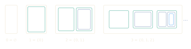

Thus evaluating finite(3) produces 𝒫(𝒫(𝒫(∅))). Its successor membership theorem is kernel checked:

x ∈ finite(succ(n)) ↔ x ⊆ finite(n)

The library also proves that every finite(n) is transitive and that finite(n) ⊆ finite(succ(n)). Both are checked theorems; the evaluator knows nothing about them.

Transfinite recursion#

ZF Foundation and Replacement justify a conservative, noncomputable class-recursion event. The surface form is:

noncomputable transfinite def V (α : Ordinal) : Set
  | 0 => ∅
  | succ β => 𝒫(V β)
  | limit λ => ⋃ { V β | β < λ }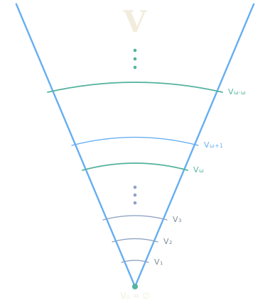

The limit comprehension is the range of a Replacement set containing the earlier pairs (β, V(β)). The kernel installs no evaluator body for V: finite executable work remains in finite, while proofs use the checked V.zero, V.next, and V.limit laws.

Clause binders have lexical scope. A general limit clause may refer directly to its index:

| limit λ => limitStep(λ, history)

The elaborator alpha-renames lambda to the definition's kernel index before the kernel checks its free variables. The history remains the only permitted route to recursive values from earlier ordinals.

Before admitting the event, the kernel unfolds the supplied Ordinal, Limit, and successor definitions and compares them with its canonical von Neumann formulas. A locally redefined predicate that happens to be named Ordinal is rejected, so the soft typing here adds nothing to the trusted foundation.

Value, DomainThrough, StageClause, Approximation, and Stage remain as a first-order graph specification of bounded approximations to the recursion

V(0)       = ∅
V(succ(β)) = 𝒫(V(β))
V(λ)       = ⋃ { V(β) | β ∈ λ }       when λ is a limit

Earlier approximation values are collected by a bounded Separation instance. CumulativeUniverse collects membership across the set-valued stages.

StageExists(α), StageUnique(α), and HierarchyResolvedThrough(α) name the exact transfinite-recursion proof obligations. Ranked is the class of sets certified to occur at some ordinal stage. The hierarchy library proves that every set belongs to it.

The Foundation library derives membership induction without a new kernel rule. It builds closure(x) as the union of the Replacement image of the finite iterates singleton(x), union(singleton(x)), ..., proves this set transitive, and proves membership restricted to it well-founded. The tactic induction x using membership expands to the existing well-founded-induction proof rule. Using it, the hierarchy library checks rank(x) ∈ Ordinal for the Foundation-recursive height

rank(x) = next(union(range(rank.history(x))))

The remaining mathematics is also derived. Foundation gives membership irreflexivity; nested membership induction gives ordinal trichotomy and the zero/successor/limit cases. The transfinite recursion history then yields

x ∈ V(λ) ↔ ∃ β ∈ λ, x ∈ V(β)

at limits. A single membership induction proves both Transitive(V(β)) and ordinal monotonicity of V, since those properties support one another at a successor. Finally rank.member_bound places every member's rank below the supremum used by rank(x), and monotonicity proves the checked theorem rank.membership : x ∈ V(rank(x)). So CumulativeUniverse.eq_Universe is an unconditional theorem; no axiom or extra recursion principle is involved.

Ordinal arithmetic#

Addition, multiplication, and exponentiation of ordinals are three more transfinite recursions, each on its right argument, with the union of the earlier values at a limit:

noncomputable transfinite def ordinalAdd (α : Ordinal, β : Ordinal) : Set
  | 0 => α
  | succ γ => next(ordinalAdd(α, γ))
  | limit λ => ⋃(Relation.range(history))

noncomputable transfinite def ordinalMul (α : Ordinal, β : Ordinal) : Set
  | 0 => ∅
  | succ γ => ordinalAdd(ordinalMul(α, γ), α)
  | limit λ => ⋃(Relation.range(history))

noncomputable transfinite def ordinalPow (α : Ordinal, β : Ordinal) : Set
  | 0 => 1
  | succ γ => ordinalMul(ordinalPow(α, γ), α)
  | limit λ => ⋃(Relation.range(history))

Under (α β : Ordinal) the operators print and parse as +, *, and ^. The laws that hold are proved by transfinite induction on the right argument, in the same way as the stage properties of V:

theorem ordinalAdd.associative (α β : Ordinal, γ : Set)
  shows γ ∈ Ordinal → (α + β) + γ = α + (β + γ)

theorem ordinalMul.distributive (α β : Ordinal, γ : Set)
  shows γ ∈ Ordinal → α * (β + γ) = α * β + α * γ

theorem ordinalPow.add (α β : Ordinal, γ : Set)
  requires positive : ∅ ∈ α
  shows γ ∈ Ordinal → α ^ (β + γ) = α ^ β * α ^ γ

The hypothesis ∅ ∈ α on the power law is not a convenience: with the recursion as written, 0 ^ ω is the union of 1, 0, 0, …, which is 1, so 0 ^ (1 + ω) ≠ 0 ^ 1 * 0 ^ ω. Addition is strictly monotone and cancellative on the right (ordinalAdd.monotone, ordinalAdd.cancel), and so are multiplication and exponentiation by an ordinal above 0 and 1 respectively; every ordinal is zero, a successor, or a limit:

theorem Ordinal.zero_successor_or_limit (α : Ordinal)
  shows α = 0 ∨ (∃ β, β ∈ Ordinal ∧ α = next(β)) ∨ Limit(α)

What fails is commutativity, and the failures are the first thing anyone learns about the ordinals. Adding one finite step before ω is absorbed:

theorem ordinalAdd.one_omega
  shows 1 + ω = ω
proof
  exact ordinalAdd.natural_omega at 1

theorem ordinalAdd.not_commutative
  shows 1 + ω ≠ ω + 1
proof
  intro equal
  have ωOrdinal := Ordinal.omega
  rw [ordinalAdd.one_omega, ordinalAdd.one] at equal
  have self := next.contains at ω
  rw ← equal at self
  exact Ordinal.not_member_self with self

The proof of the inequality is the whole story: 1 + ω is ω by absorption and ω + 1 is next(ω), which contains ω, so equality would make ω a member of itself. Multiplication and exponentiation behave the same way (ordinalMul.two_omega, ordinalMul.not_commutative, ordinalPow.two_omega):

theorem ordinalMul.two_omega
  shows 2 * ω = ω
proof
  have positive : ∅ ∈ 2
    apply membership.two.backward
    left
    symm
    exact nat.zero
  exact ordinalMul.natural_omega at 2 with positive

theorem ordinalPow.two_omega
  shows 2 ^ ω = ω
proof
  have above : 1 ∈ 2
    apply membership.two.backward
    right
    rfl
  exact ordinalPow.natural_omega at 2 with above

Every theorem in these modules audits as ZF alone.

Every set has a rank#

The stages of the hierarchy exhaust the universe: every set lies in some V(α). In Cumulus this is the class equality CumulativeUniverse = Universe, and the argument is a page of ordinary mathematics over two transfinite definitions. This section walks through it, with the proofs as they are checked in Hierarchy.g17.

Two recursions#

The first definition is V, by recursion on the ordinals, as above. The second is the rank function, by recursion on membership. Foundation makes ∈ well-founded, so a definition may consult its own values at the members of its argument; the keyword foundation asks for exactly that, and history is the Replacement graph of those earlier values:

noncomputable foundation def rank (x : Set) : Set
  | x using history => next(⋃(Relation.range(history)))

So rank(x) is the successor of the supremum of the ranks of the members of x. That it is an ordinal is the first theorem, by membership induction, and that membership lowers rank is the second, which is the whole interface a user of rank needs:

theorem rank.member (y x : Set)
  requires hy : y ∈ x
  shows rank(y) ∈ rank(x)
proof
  simp [rank.member_bound, rank.unfold]

induction x using membership is membership induction: the Foundation library builds the transitive closure of x as the union of the finite iterates of ⋃, proves membership well-founded on it, and the tactic expands to the kernel's well-founded induction rule.

One induction for transitivity and monotonicity#

The two facts about V that the rank argument needs are that each stage is a transitive set and that the stages grow along the ordinals. Neither is provable alone at a successor stage: 𝒫(V(β)) is transitive because V(β) is transitive and contains the earlier stages, and V(α) ⊆ 𝒫(V(β)) for α ≤ β because the earlier stages are transitive. So they are proved together, by one membership induction over the index:

theorem V.transitive_and_monotone (β : Set)
  shows β ∈ Ordinal → (Transitive(V(β)) ∧ (∀ α, α ∈ Ordinal → α ∈ next(β) → (V(α) ⊆ V(β))))

The proof is a case split on zero, successor, and limit, each case a few lines of simp and apply over the three laws V.zero, V.next, and V.limit; V.transitive and V.monotone read the two conjuncts off it. At a limit, membership in the stage is membership in some earlier stage:

theorem V.limit_membership (x λ : Set)
  requires hLimit : Limit(λ)
  shows x ∈ V(λ) ↔ ∃ earlier ∈ λ, x ∈ V(earlier)

The rank argument#

Now we can prove that every set lies in the hierarchy, at the stage given by its rank:

theorem rank.membership (x : Set)
  shows x ∈ V(rank(x))
proof
  induction x using membership
  intros current ih
  rw rank.unfold
  have hSupremumOrdinal := rank.supremum_ordinal at current
  have hSuccessorEquation := V.next with hSupremumOrdinal
  rw hSuccessorEquation
  apply set.powerset.backward
  intros member hMember
  have hMemberRanked := ih with hMember
  have hMemberBound := rank.member_bound with hMember
  have hMonotone := V.monotone at rank(member), ⋃(Relation.range(rank.history(current))) with rank.ordinal at member, hSupremumOrdinal, hMemberBound
  exact hMonotone with member, hMemberRanked

By membership induction, every member of current lies in the stage of its own rank. rank(current) unfolds to the successor of the supremum s of the members' ranks, and V(next(s)) is 𝒫(V(s)), so it suffices that every member lies in V(s). A member lies in V(rank(member)) by the induction hypothesis, its rank is at most s by rank.member_bound, and V is monotone, which finishes. Nothing is hidden in automation here: simp never runs, and each have names the fact it uses.

The universe is the hierarchy#

CumulativeUniverse is the class of sets that occur at some stage, and Universe the class of all sets. Classes are predicates on sets, so an equality between them is an extensional statement that the kernel checks pointwise:

class CumulativeUniverse (x : Set) := { x | ∃ α, α ∈ Ordinal ∧ x ∈ V(α) }

theorem rank.exists (x : Set)
  shows ∃ α, α ∈ Ordinal ∧ x ∈ V(α)
proof
  refine ⟨rank(x), rank.ordinal at x, rank.membership at x⟩

theorem CumulativeUniverse.eq_Universe
  shows CumulativeUniverse = Universe
proof
  apply CumulativeUniverse.eq_Universe_of_rank
  intro x
  exact rank.exists

The witness for the existential is the rank itself. The axiom audit of CumulativeUniverse.eq_Universe lists the ZF axioms, Foundation among them, and nothing else: no choice, no reflection, no extra recursion principle. The two recursion keywords, transfinite and foundation, are not axioms either. Each is justified once, by Replacement and well-foundedness, and the kernel admits a recursive definition only after unfolding the Ordinal, Limit, and successor predicates it was given and comparing them with its own von Neumann formulas.

Cantor's derived sets#

The ordinals were discovered in 1872, in Cantor's study of the sets on which a trigonometric series can fail to determine its coefficients. The derived set of a set of reals is the set of its limit points; the derived set of the derived set is a smaller set again; and Cantor saw that the iteration need not stop at any finite stage, which leads directly into the transfinite. The theorem that grew out of this, the Cantor–Bendixson theorem, says that every closed set of reals is a perfect set together with a countable set. Cumulus proves it for every space with a countable base, by effectively the same approach as the rank argument above: a transfinite recursion, and an induction along it. The modules are Topology/CantorBendixson and Topology/Real/CantorBendixson.

The iteration#

derivedSet(X, T, A) is limitPoints(X, T, A), the points of X every open neighbourhood of which meets A elsewhere. The stages are a transfinite recursion, with intersection at limits:

noncomputable transfinite def derived (X T A : Set, α : Ordinal) : Set
  | 0 => A
  | succ β => derivedSet(X, T, derived(X, T, A, β))
  | limit λ => ⋂(Relation.range(history))

The three laws derived.zero, derived.next, and derived.limit state the three clauses as equations, and at a limit a point survives exactly when it survives every earlier stage:

theorem derived.limit_membership (X T A x λ : Set)
  requires limit : Limit(λ)
  shows x ∈ derived(X, T, A, λ) ↔ ∀ β ∈ λ, x ∈ derived(X, T, A, β)

For a closed set the stages are closed and decrease along the ordinals (derived.closed, derived.decreasing), each by one induction over the index.

Why the iteration stops#

A point leaves at stage γ when it is isolated in derived(γ): some basic open set W meets that stage in the point alone. The same W cannot witness two departures, at the same stage or at different ones, because the stages decrease:

theorem derived.witness_injective (X T A B γ δ x y W : Set)
  requires topology : IsTopology(X, T)
  requires basis : Basis(X, T, B)
  requires closed : IsClosed(X, T, A)
  requires hGamma : γ ∈ Ordinal
  requires hDelta : δ ∈ Ordinal
  requires hW : W ∈ B
  requires first : W ∩ derived(X, T, A, γ) = {x}
  requires second : W ∩ derived(X, T, A, δ) = {y}
  shows γ = δ ∧ x = y

So if the base B is countable, the stages cannot keep dropping for uncountably many steps. Hartogs' bound hartogsBound(B) is the least ordinal that does not inject into B; if every stage below it dropped, the witnesses would give such an injection. The proof picks each witness as the one of least code under the injection of B into ℕ, so no choice is used:

theorem derived.stabilises (X T A B : Set)
  requires topology : IsTopology(X, T)
  requires basis : Basis(X, T, B)
  requires closed : IsClosed(X, T, A)
  requires countable : Countable(B)
  shows ∃ γ ∈ hartogsBound(B),
    derived(X, T, A, next(γ)) = derived(X, T, A, γ)
proof
  obtain ⟨g, code⟩ := countable
  by_contra none
  have hBound := hartogsBound.ordinal at B
  have ordinals : ∀ γ ∈ hartogsBound(B), γ ∈ Ordinal
    intros γ hγ
    exact Ordinal.member with hBound, hγ
  have offered : ∀ γ ∈ hartogsBound(B), ∃ W ∈ B,
      relates(stageDrops(X, T, A, B, hartogsBound(B)), γ, W)
    intros γ hγ
    have hGamma := ordinals with γ, hγ
    have strict : derived(X, T, A, next(γ)) ≠ derived(X, T, A, γ)
      intro equal
      apply none
      exact ⟨γ, hγ, equal⟩
    obtain ⟨W, hW, x, trace⟩ := stageDrops.offered with
      topology, basis, closed, hGamma, strict
    witness W
    constructor
    . exact hW
    . apply stageDrops.relates.backward
      exact ⟨hγ, hW, x, trace⟩
  have separated := stageDrops.separated with topology, basis, closed, ordinals
  have injective := leastCoded.injective with code, offered, separated
  exact hartogsBound.no_injection with injective

The Cantor–Bendixson rank is the least stable stage, and the kernel is the stage there:

def stableStages (X T A : Set) : Set :=
  { γ ∈ hartogsBound(T) | derived(X, T, A, next(γ)) = derived(X, T, A, γ) }

def cantorBendixsonRank (X T A : Set) : Set := ⋂(stableStages(X, T, A))

def perfectKernel (X T A : Set) : Set :=
  derived(X, T, A, cantorBendixsonRank(X, T, A))

The theorem#

A perfect set is a closed set equal to its derived set, a closed set without isolated points:

predicate Perfect (X T P : Set) := IsClosed(X, T, P) ∧ derivedSet(X, T, P) = P

theorem cantorBendixson (X T B A : Set)
  requires topology : IsTopology(X, T)
  requires basis : Basis(X, T, B)
  requires closed : IsClosed(X, T, A)
  requires countable : Countable(B)
  shows Perfect(X, T, perfectKernel(X, T, A)) ∧
    perfectKernel(X, T, A) ⊆ A ∧ Countable(A ∖ perfectKernel(X, T, A))

The kernel is perfect because it is a stable stage; it lies in A because the stages decrease; and the points of A outside it each left at some stage below the rank, with a witness in B, so they inject into B and are countable. The rank itself is a countable ordinal (cantorBendixson.rank_countable). The axiom audit of every one of these theorems lists the ZF axioms and nothing else.

On the real line#

The open intervals with rational endpoints are a countable base of the real topology (rationalIntervals.basis, with the density of ℚ in ℝ proved from the cut structure of the reals), so the theorem specialises:

theorem reals.cantorBendixson (A : Set)
  requires closed : IsClosed(ℝ, realTopology, A)
  shows Perfect(ℝ, realTopology, perfectKernel(ℝ, realTopology, A)) ∧
    perfectKernel(ℝ, realTopology, A) ⊆ A ∧
    Countable(A ∖ perfectKernel(ℝ, realTopology, A))

theorem closed.countable_or_perfect_part (A : Set)
  requires closed : IsClosed(ℝ, realTopology, A)
  shows Countable(A) ∨
    (∃ P, Nonempty(P) ∧ Perfect(ℝ, realTopology, P) ∧ P ⊆ A)

A nonempty perfect set of reals is uncountable, by Cantor's nested intervals: around a point of the set, every interval meets the set again, so a shrinking sequence of closed intervals can be chosen that stays in the set and avoids each enumerated point in turn, and its common point is in the set but in no position of the enumeration. The choice of intervals is where the axiom of choice enters, and it is the only place.

theorem perfect.uncountable (P : Set)
  requires perfect : Perfect(ℝ, realTopology, P)
  requires nonempty : Nonempty(P)
  shows ¬Countable(P)

theorem closed.countable_or_uncountable_perfect (A : Set)
  requires closed : IsClosed(ℝ, realTopology, A)
  shows Countable(A) ∨
    (∃ P, Nonempty(P) ∧ Perfect(ℝ, realTopology, P) ∧ P ⊆ A ∧
      ¬Countable(P))

This is Cantor's beautiful conclusion, obtained with the power of the ordinals: a closed set of reals is countable or contains a nonempty perfect set. You might find it as thrilling as I do to click "Open in Workbench" on any of the snippets above to follow the argument yourself!